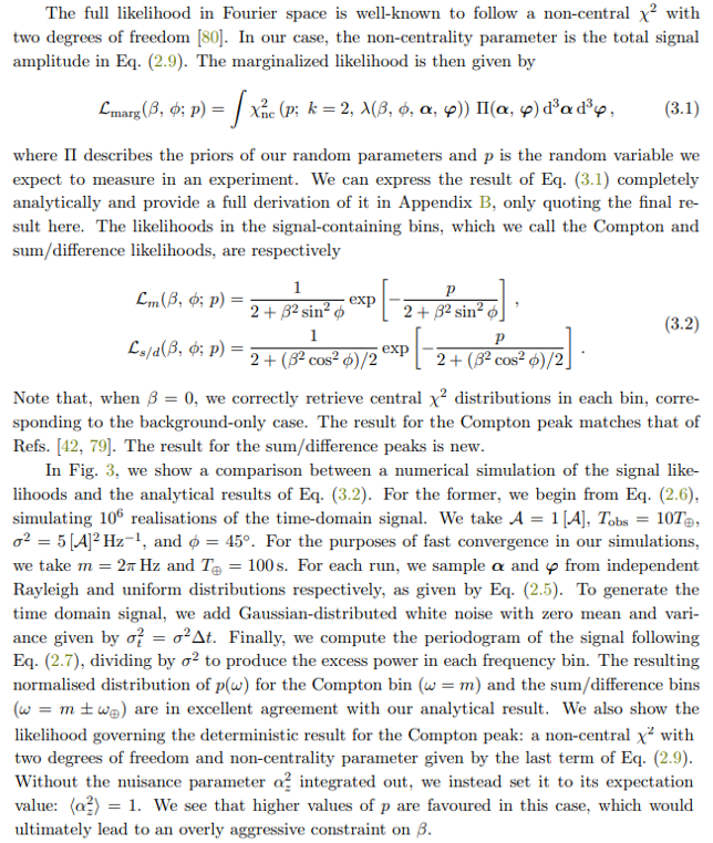
Authors:
(1) Dorian W. P. Amaral, Department of Physics and Astronomy, Rice University and These authors contributed approximately equally to this work;
(2) Mudit Jain, Department of Physics and Astronomy, Rice University, Theoretical Particle Physics and Cosmology, King’s College London and These authors contributed approximately equally to this work;
(3) Mustafa A. Amin, Department of Physics and Astronomy, Rice University;
(4) Christopher Tunnell, Department of Physics and Astronomy, Rice University.
Table of Links
2 Calculating the Stochastic Wave Vector Dark Matter Signal
3 Statistical Analysis and 3.1 Signal Likelihood
4 Application to Accelerometer Studies
4.1 Recasting Generalised Limits onto B − L Dark Matter
6 Conclusions, Acknowledgments, and References
A Equipartition between Longitudinal and Transverse Modes
B Derivation of Marginal Likelihood with Stochastic Field Amplitude
D The Case of the Gradient of a Scalar
3 Statistical Analysis
We now consider the projected exclusion limits that a generic experiment would be able to set using our three-peak analysis. To do this, we use a series of likelihood-ratio tests.
3.1 Signal Likelihood
For our likelihood, we follow a hybrid frequentist-Bayesian approach, defining a marginalized likelihood in which all nuisance parameters are integrated out. In our case, these are the random Rayleigh parameters, α, and random uniform DM phases, φ. Such a hybrid approach has already been used in the context of ultralight bosonic dark matter [42, 79]. Our work differs from Ref. [79] since they focused on an axion-like signal as opposed to that from vector DM. It goes beyond Ref. [42] since they did not consider the peaks arising from the rotation of the Earth in their analysis.


The full likelihood over all frequency space is then given by the product of the likelihoods in each frequency bin,

where pi represents the excess power density in the ith frequency bin, p is the full data vector, and the product runs over all Nbins frequency bins. Ultimately, since our signal only manifests in three bins, it suffices for us to consider only those bins that could potentially contain a signal, and we may ignore all other bins. We can express the likelihood in this way because each bin is statistically uncorrelated, as we show in Appendix C. This is in contrast with the analysis performed in Ref. [45], where a similar study was conducted in the case of the gradient of a scalar in the time domain. There, a complicated covariance matrix had to be computed to account for correlations in the signal at different times. In Fourier space, these covariances disappear. The power of performing this analysis in the frequency domain is thus not only that the signal is contained within a small number of bins, but also that these bins are statistically independent, which allows us to treat the statistics in a significantly simpler way.
Crucially, once the latitude of the experiment, ϕ, is fixed, the likelihood depends on the product of all experimental variables via the dimensionless parameter β. This means that we can set a more holistic limit that is independent of the specifics of an experiment. Once the form of A (which depends on both the experiment and the DM model), the observation time Tobs, and the noise profile σ are known, the ensuing limit on β can be recast to one on the model parameters of interest. This makes our analysis, both the results and overall logic, as generally useful as possible.
This paper is available on arxiv under CC BY 4.0 DEED license.

